Distributing principal components

The Principal Component Analysis (PCA), a compression method widely used in statistical anaylsis and image processing, can be efficiently implemented in a network of wireless sensors. PCA proves to be particularly suitable to sensor networks as it allows to reduce the network load while retaining a maximum amount of variance from sensor measurements. At least two operating modes can be designed, unsupervised and supervised, allowing (i) to extract a maximum of variance while keeping the network load bounded, and (ii) to reduce the network load while keeping the approximation error bounded, respectively (work sumbitted). The current purpose of this research track is to design a fully distributed implementation for the computation of the principal components.

Student involved: Sylvain Raybaud

References:

[1] A. Hyvarinen, J. Karhunen, and E. Oja. Independent Component Analysis. J. Wiley New York, 2001.

[2] K. Diamantaras and S. Kung. Principal component neural networks: theory and applications. John Wiley
& Sons, Inc. New York, NY, USA, 1996.

[3] I. Jolliffe. Principal Component Analysis. Springer, 2002.

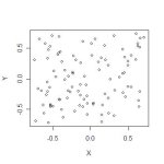
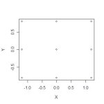
Localization

The goal of this project is to study and share experimental results obtained for the localization problem using TMote Sky wireless sensors, whose CC2420 radio is compliant with the IEEE 802.15.4 emerging standard for WSN. Using multidimensional scaling (MDS), considered as a competitive algorithm for localization in WSN, we compare localization performances obtained with CC2420 radio by using RSSI (Received Signal Strength Indicator) and LQI (Link Quality Indicator) as indicators for estimating sensor nodes pairwise distances. While RSSI has been part of low power radio hardware for a few years, and is the indicator usually used for localization, LQI is more recent, and few studies have so far compared these indicators in localization problems.

Ongoing experiments also aim at automatically tuning the transmission power of the CC2420 radio to different levels in order to improve the localization accuracy.

Student involved: Mathieu Van Der Haegen

Download data and code from the master thesis. It includes:

TinyOS code for obtaining RSSI and LQI indicators
Java code to interface the wireless sensor network
All the datasets collected (RSSI and LQI for different radio transmission powers - 20 sensor nodes)

References:

[1] J. Costa, N. Patwari, and A. Hero. Distributed multidimensional scaling with adaptive weighting for node localization in sensor networks. ACM Transactions on Sensor Networks (TOSN), vol. 2, no. 1, pp. 39–64, 2006.

[2] K. Whitehouse and D. Culler. A robustness analysis of multi-hop ranging-based localization approximations. Proceedings of the fifth international conference on Information processing in sensor networks, pp. 317–325, 2006.

[3] Presentation at Machine Learning Group - December 2006 (in French). [PDF]

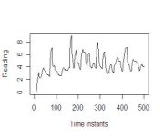
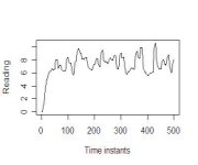
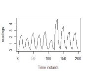
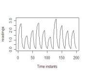
Prediction models for wireless sensor networks

Use of prediction models in sensor networks proves to be efficient with respect to energy savings, as it allows sensors whose readings are predicted to remain in their idle mode, thereby consuming orders of magnitude less energy that in the active mode. In the context of continuous monitoring, where a set of sensors is typically required to regularly send their readings to a central server, an interesting approach consists in splitting the set of sensors in two subsets, such that readings of one subset are used to predict readings of the second subset. An approach for finding such a subset was proposed in [1].

This project pursues this research track, the goal is to identify several sensor subsets for predictions, that are used in turn in a round robin fashion. Identification of different sensor subsets allows to detect erroneous models or sensor failure, and to better distribute energy consumption. More detailed can be found in [2], and in the following presentation [3].

References:

[1] A. Desphande, C. Guestrin, S. R. Madden, J. M. Hellerstein, and W. Hong. Model-driven data acquisition in sensor networks, Proceedings of the 30th VLDB Conference, Toronto, Canada, 2004. [PDF]

[2] Y. Le Borgne, G. Bontempi. Round Robin Cycle for Predictions in Wireless Sensor Networks.
To appear in: 2nd International Conference on Intelligent Sensors, Sensor Networks and Information Processing (ISSNIP 2005), December 2005, Melbourne, Australia. [PDF]

[3] UCL Microelectronics course, Louvain La Neuve, Belgium - February 2006. [PDF]

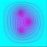
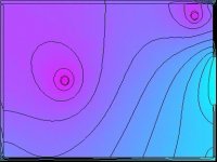
Environmental modeling for synthetic data generation

As real world deployments of wireless sensor networks (WSN) are cost and time consuming, few real world data sets exist for assessing data processing architectures for WSN. Goal of this work is to use PDEs to provide realistic synthethic datasets for testing WSN data processing algorithms.

A large panel of natural environmental variations, such as temperature, humidity, chemicals concentration, vibrations, pressure, and so forth, can be modelled by using adequate sets partial differential equations. These page currently provides some examples and MATLAB codes we used for generating data of diffusion processes.

Diffusion processes:

Diffusion processes can be modelled by the following parabolic equation:

Where V(x,t) is the measure of interest (over space and time), D the diffusion coefficient and Q the medium activity. For example, for heat propagation, D would be the heat diffusivity and Q the ratio of the heat source in Joule over the heat capacity of the medium. Construction of an environment requires associating to each element of the environment adequate D and Q parameters, and defining boundary conditions for the outer boundaries (Dirichlet or Neumann conditions).

Scenarios:

These examples were done using the MATLAB Partial Differential Equation toolbox.

Example 1)

The environment is a square region with Dirichlet boundaries set at zero (so that the borders are kept at a constant temperature, simulating an open environment). Three diffusion sources move randomly at 50 sets of positions within the environment, and data was collected for ten time instants for each sensor positions. Here, 100 sensors were randomly placed over the environment (see figure 1 below). Diffusion parameters were set so as to observe variations of about ten units over time in the measured physical quantity (see figures 2 for the sensor situated at the center of the environment, and figure 3 for the sensor situated at the top left corner).

Collected data, together with positions of heat sources and sensors are available here.

Matlab code is available here. A change of only few parameters allow to generate varying number of heat sources or sensors.

Video (9MB)


1) Sensor map	2) Sensor (center) readings	3) Sensor (top left) readings

Example 2)

Here we simulated apperance and disappearance of heat sources in a closed rectangular environment with one operture and heat dissipation on the boundaries. Heat dissipation is obtanied by adding on the boundaries a layer with a lower diffusion coefficient than that of the inside of the environment. The operture on the the right hand side is obtained by removing locally this layer. Number of heat sources varies from 1 (video 1 on the right) to 3 (video 3), with 10 sets of different heat source locations for each condition.

For each set of location, temperature increase is observed for a period of ten time instants. Sources are the removed, and temperature decrease is observed for another tentime instants. Readings are collected by a set of nine sensors arranged in a grid (see figure 1 below). Example of collected temperature readings are reported on figure 2 and 3 below.

An archive containing the generated data sets is available here, and corresponding Matlab code can be found here.


Video 1 (2MB)	Video 2 (2MB)	Video 3 (2MB)


1) Sensor map	2) Sensor (center) readings	3) Sensor (top left) readings

Contact person: Yann-Aël Le Borgne - Machine Learning Group - ULB Computer Science Department